Analysis of Variance (most commonly referred to as ANOVA) is a common statistical test that compares the averages of several sets of data. It is unlikely for datasets to have the same average, and an ANOVA test quantifies how likely those observed differences in occurred by chance. It is a really useful test because we frequently find ourselves comparing averages of different datasets. We may, for example, compare the average customer demand for different months, or the average turnaround time for several job shops, or the average length of stay for hip replacement patients for several different doctors. These comparisons are useful because they can give us insight into the underlying value streams. If the length of stay varies from physician to physician, it might suggest an underlying variation in the treatment protocol. If customer demand varies from month to month, is the variation just noise or are the observed differences in average customer demand unlikely to have occurred by chance? And if they are unlikely to have occurred by chance, what is causing the change in demand? Are your competitors having sale events that you aren’t? An ANOVA analysis won’t tell you why the averages are different, but it will signal if something unusual is going on that warrants further investigation. The steps for performing an ANOVA analysis are as follows: Step 1: Look at the data. Do the data points look reasonable? Are the values high or low (good or bad)? How do the values compare to expectations? How do they compare to benchmarks? Are there any outliers or anomalous values? Do the averages appear different? What factors distinguish the datasets? Step 2: Make several different graphs comparing the different datasets (e.g. Dot Plot, Boxplot, Histogram, and Interval Plot). Do the datasets appear to have the same averages? Do the datasets appear to be normally distributed and have the same variance? Step 3: Verify the prerequisites of ANOVA analysis. Test the normality of the datasets. Test for equal variances. (If the prerequisites are not satisfied, there are several options: transform the data; proceed with the ANOVA analysis and use the results with appropriate caution; or use a different hypothesis test e.g. Mood’s Median or Kruskal-Wallis and compare medians instead of averages). Step 4: Run the ANOVA analysis and analyze the results. The null hypothesis (H0) of an ANOVA analysis is that the means are equal, if the p Value is low, the statistical conclusion is that the difference in the means is statistically significant (i.e. unlikely to have occurred by chance). Step 5: Examine the residuals, and summarize the results. Example: A few car enthusiasts are testing the impact that a fuel additive has on their fuel mileage. They ran 10 trials, with 10 gallons of gas each, and the change of their miles per gallon was as follows:
| Nova | Chevy 1 | Chevy 2 | Ford |
| -0.9 | 0.2 | 2.5 | -0.8 |
| -0.7 | 0.2 | 0.8 | 1.0 |
| -1.1 | -0.2 | 1.1 | -0.6 |
| 1.2 | -1.1 | 1.8 | -0.2 |
| -0.1 | 0.3 | 1.8 | -2.1 |
| -0.1 | 0.4 | 2.9 | -0.3 |
| 0.0 | -0.8 | 0.7 | 0.6 |
| 0.8 | 0.8 | 2.7 | -2.7 |
| 1.1 | 0.0 | 1.8 | -0.2 |
| -0.2 | -0.9 | 0.7 | -0.6 |
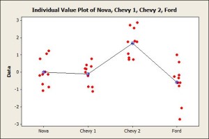
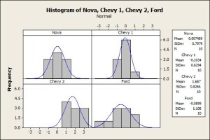
Step 1: Looking at the data. Here, we don’t see much other than all of the values for Chevy 2 are positive, indicating that for each trial the miles per gallon increased. Step 2: Graph the data. Here again we see that the average for Chevy 2 appears to be the highest.  Step 3: Validate the assumptions for an ANOVA analysis. Two of the assumptions for an ANOVA analysis are that the datasets are normally distributed and have equal variances. The histograms are consistent with these assumptions, and statistical tests such as the Anderson-Darling normality test and Bartlett’s test for equal variances also yield results that are also consistent with these assumptions.
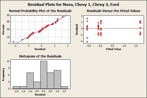
  Step 4: Run the ANOVA analysis. Any reasonable statistical software can do this for you. Our software gave us a p-value (i.e. the likelihood that the observation occurred by chance), of 0.000 indicating that the results are statistically unusual. Step 5: Examine the residuals and summarizing the analysis. A residual is the part of each data value that is not explained by the model. Where the model is simply the observed data is equal to the overall data average plus a column average offset.
  There are no obvious patterns to the residuals, so our conclusion is that the mpg increase for Chevy 2 was unexpected. Subsequent conversations with the Chevy 2 driver revealed that they emptied their trunk, properly inflated their tires, and accelerated more gently for the test. All of which may explain the observed result. The point being that with analysis we gain insight into hidden, underlying process dynamics.
